IQ modulator demo (supplementary material)#
IQ modulator is widely used in coherent optical communications.
We can use an IQ modulator to generate signals with advanced modulation formats such as QPSK, and m-QAMs.
What we are going to learn in this notebook#
Understand how I/Q modulator works
Generate I/Q signals, use numpy function ‘fft’ for Discrete Fourier Transform.
Apply I/Q signals to I/Q modulator model
Plot output signals
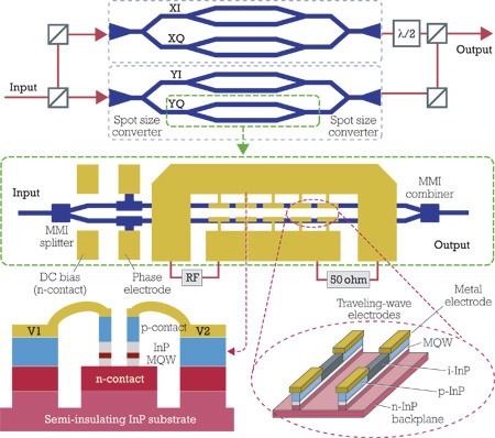
How I/Q modulator works#
from IPython.display import Image
from IPython.core.display import HTML
Image(url="https://img.lightwaveonline.com/files/base/ebm/lw/image/2015/12/1503lwcovrstoryf2.png?auto=format&w=1500&h=843&fit=max")
Generate I/Q signals#
pattern mapping
raised cosine filter for pulse shaping (roll-off factor 0.2)
%pylab inline
def makeQAMtarget(shift=0.,N = 2**31,BaudRate = 30, BD=2,beta=.1,half=False,pat_en=None,ModNumber=2,get_rid_DC=None,DEBUG = False):
"""
In this particular example, we generate 16-QAM signals.
We can also generate M-QAM signals.
"""
if pat_en is None:
Np = int((N)/BD)
random.seed(103231)
pattern = (random.randn(Np)>0) + 1j*(random.randn(Np)>0) # QPSK
pattern -= .5+.5j
p1 = (random.randn(Np)>0) + 1j*(random.randn(Np)>0)
p1 -= .5+.5j
pattern += p1*.5 # 16QAM
p1 = (random.randn(Np)>0) + 1j*(random.randn(Np)>0)
p1 -= .5+.5j
#pattern += p1*.25 # 64QAM
else:
pattern1=io.loadmat(pat_en)
pattern = pattern1['a'][:,0]
pattern -= np.mean(pattern)
pattern /=(mean(abs(pattern)**2))**0.5
if ModNumber==1:
pattern=roll(pattern,len(pattern)//2)
SampleRate = 2.*BaudRate
br = BD/SampleRate
N = int(len(pattern)*BD)
f = arange(-N/2,N/2)/N*SampleRate
e = zeros(N,complex)
e[::int(BD)] = pattern
s = fft.fftshift(fft.fft(e))
#plot(f,)
shaping_filter = RCFilter(beta,f,br)
if DEBUG:
figure(figsize = (5,2))
plot(f,shaping_filter)
s *=shaping_filter
if half:
s*= f>0
if get_rid_DC:
s*= abs(f)>10
#pre-emphasis for dac roll off
et = fft.ifft(fft.fftshift(s))
et /= mean(abs(et)**2)**.5
return f,et,pattern
def RCFilter(beta,f,T):
"""
raised-cosine filter for pulse shaping
"""
H = zeros(len(f),dtype = complex)
finner = abs(f)<=((1-beta)/2./T)
fmiddle = (abs(f)>=((1-beta)/2./T))&(abs(f)<=((1+beta)/2./T))
H[finner] = 1
H[fmiddle] = 1./2*(1+cos(pi*T/beta*(abs(f[fmiddle])-(1-beta)/2./T)))
return H
## et is
f,et,pattern = makeQAMtarget(shift = 0.,
N = 2**15,
BaudRate = 30.,
BD = 2.,
beta = 0.2,
half = False,
DEBUG = False)
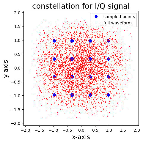
figure(1,figsize = (5,5))
plot(real(et[::2]),imag(et[::2]),'bo',label = 'sampled points')
plot(real(et),imag(et),'r,',label = 'full waveform')
title('constellation for I/Q signal',fontsize = 18)
xlabel('x-axis',fontsize = 15)
ylabel('y-axis',fontsize = 15)
legend()
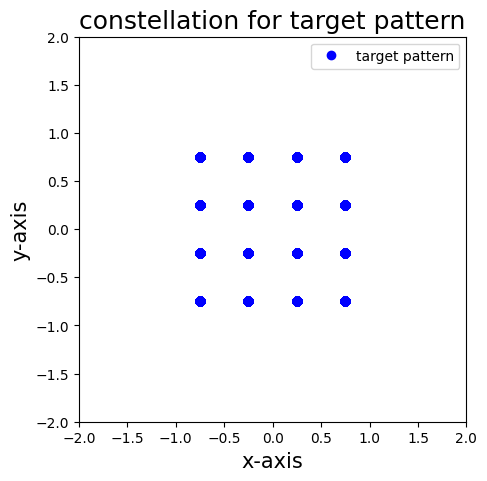
figure(2,figsize = (5,5))
plot(real(pattern),imag(pattern),'bo',label = 'target pattern')
title('constellation for target pattern',fontsize = 18)
xlabel('x-axis',fontsize = 15)
ylabel('y-axis',fontsize = 15)
xlim(-2,2)
ylim(-2,2)
legend();
%pylab is deprecated, use %matplotlib inline and import the required libraries.
Populating the interactive namespace from numpy and matplotlib
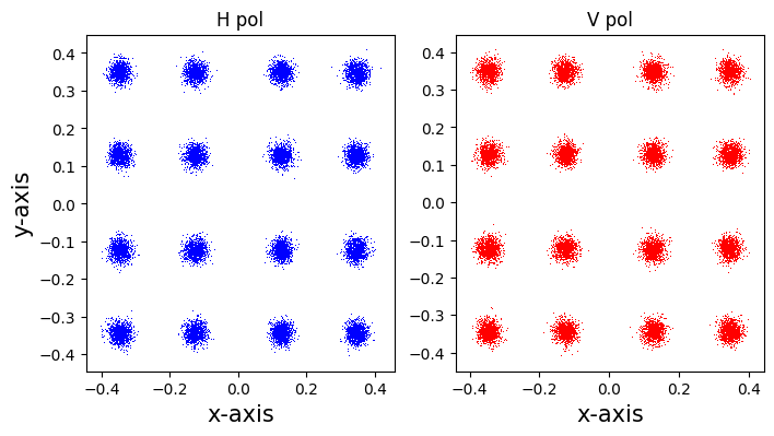
Apply generated signals to I/Q modulator model#
practical model includes modulator bias, 90 degree phase shifter, Vpi, Driver amplitude and OSNR
practical model includes polarization modulator (here we assume time-invariant polarization shift).
Plot output signals#
def Pol_Emu(e_te,e_tm,theta,baudrate):
    """
    polarization emulator (only with time-invariant polarization shift)
    e_te: TE signal
    e_tm: TM signal
    theta: polarization rotating angle
    """
    N = len(e_te)
    dt = 1./2/baudrate
    t = arange(0,N)*dt
    c  = cos(theta)
    s = sin(theta)

    eH = e_te*c+e_tm*s
    eV = -e_te*s+e_tm*c

    return eH,eV

def TX_SIMU(efull,N = 2**15,Bias_I = 0.,Bias_Q = 0.,TX_90 = pi/2.,Driver_Amp = 2,Vpi = 4.,OSNR = 20.,theta = 0.):
    '''
    et is the full pattern
    N is the data length that we used for the pattern, and it started with a initial value
    Bias_I is the bias phase shifter of the I side
    Bias_Q is the bias phase shifter of the Q side
    TX_90 is the phase shifter of 90 degree phase shifter
    Driver_Amp is the driver output amplitude
    Vpi is the Voltage needed for pi phase shift of the MZM (I/Q)
    '''
    initial_index = mod(floor(random.randn()*2**15),2**15)
    if mod(initial_index,2) == 1:
        initial_index -= 1

    initial_index = int(initial_index)
    e = efull[initial_index:initial_index+N]
    Ph_I = real(e)*Driver_Amp+Bias_I
    Ph_Q = imag(e)*Driver_Amp+Bias_Q

    eout = 0.5*(sin(0.5*Ph_I/Vpi*pi)+exp(1j*TX_90)*sin(0.5*Ph_Q/Vpi*pi))
    eout1 = roll(eout,380)

    ### need to add AWGN based on OSNR (default is 20 dB)
    GBB_temp = 10**((OSNR-10*log10(30.*2./12.5))/10.)
    power_noise = mean(abs(eout)**2.)**.5/(1+GBB_temp)
    print(power_noise)
    noise_add = (random.randn(N)+1j*random.randn(N))*power_noise
    noise_add1 = (random.randn(N)+1j*random.randn(N))*power_noise
    eout_awgn = eout + noise_add
    eout_awgn1 = eout1 + noise_add1

    eH,eV = Pol_Emu(eout_awgn,eout_awgn1,theta,30)

    return eH,eV
e_full = tile(et,2**6) ### repeat et for 2**6 times
Eout_H,Eout_V = TX_SIMU(efull = e_full,
                        N = int(2**15),
                        Bias_I = 0,
                        Bias_Q = 0,
                        TX_90 = pi/2.,
                        Driver_Amp = 1.,
                        Vpi = 2.,
                        OSNR = 20.,
                        theta = 0.)

figure(1,figsize = (8,4))
subplot(121)
plot(real(Eout_H[::2]),imag(Eout_H[::2]),'b,')
title('H pol')
xlabel('x-axis',fontsize = 15)
ylabel('y-axis',fontsize = 15)

subplot(122)
plot(real(Eout_V[::2]),imag(Eout_V[::2]),'r,')
title('V pol')
xlabel('x-axis',fontsize = 15);
0.016226785771489192