A basic introduction to Python#

While it is not possible to give a full introduction to Python in the short time for this course, we aim here to give a brief introduction into some of the main features that are important for the rest of the course. If you have never used Python before we recommend to familiarize yourself before the course using one of the many excellent resources on the net, like the official Python Tutorial

Learning Outcomes#

A basic understanding of the Python programming language
Learn how to install Python using Miniforge
Learn about basic types and their usage
Learn how to write and use functions and classes
What are modules and how to use them
Why you should almost always use Numpy

Why Python#

Trend based on Github users #

top

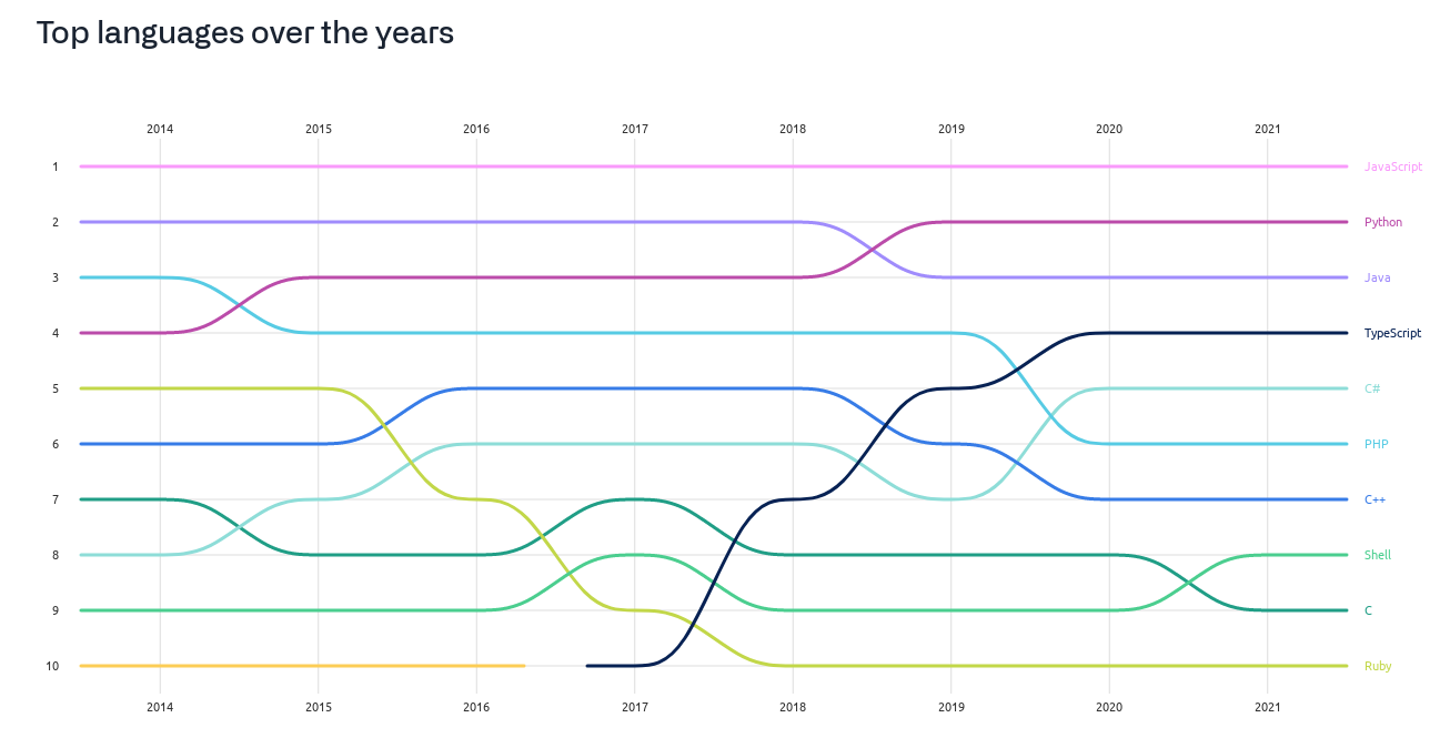
Why did we choose Python for our Labautomation and why should you#

Python is a free open source programming language with a straight forward syntax. Some of the advantages offered by Python are:

Easy to learn (many educational resources)
Runs on many platforms (from PC to raspberry pi to BBC microbit)
Excellent numerical and scientific tools
General purpose programming language (use it for simulations, lab-automation, scripts, GUIs…)
Easy to read (difficult to write hard to understand code)
It’s fun!

For lab-automation it is particularly powerful that Python has a simple approach to object-oriented programming and that it support an easy interface with other programming language like C, Fortran and CUDA.

How to install Python (Everyone starts from here)#

One of the initially confusing aspects of Python is how to get everything you need installed.

Python is separated into the core language and modules which can be regarded as the equivalent to libraries in C. The default Python language install contains a large standard library with modules covering everything from regular expressions pattern matching to logging and web parsing. However the important modules for numerical/scientific work are not part of the standard library

While it is possible to install all required modules manually it is usually desired to instead install a Python distribution, which has all modules already installed.

There are several excellent python distributions available, in this shortcourse we will use Miniforge, as it is freely available without any restriction. If commercial support is desired a common popular distribution available is Anaconda

We highly recommend using a python distribution like Minforge or Anaconda, particularly for Windows or MAC OS user, whereas Linux users are often also well served by the Python installation and Python add-on packages offered by the system package-manager.

Installation#

Installing Miniforge is straight forward

Download the Miniforge3 installer for the appropriate operating system from here
Follow the installation instructions on the web page
- For Windows: Double click on the downloaded file and accept all defaults settings in the installer
- For Linux: Run bash Miniforge3-Linux-x86_64.sh followed by ~/miniforge3/condabin/conda init
Add additional packages using the conda command as described in section 3
Additional instructions for more advanced installations can be found in Miniforge install

Installation of the following packages are required for the shortcourse:

numpy
scipy
matplotlib
spyder
jupyterlab
pyVISA

This can be achieved with the following command: conda install numpy scipy matplotlib spyder jupyterlab pyVISA

Alternative python environment for this class: google colab #

Programming Python#

Writing python programs can be done in two different ways

interactively
non-interactively

What to use for programming depends on the user case. For interactive programming you can directly start the python interpreter and begin programming. However, the default interpreter is relatively bare, the two recommended ways for interactive use, which are both installed with Anaconda, are:

The IPython console (a much more feature-full interpreter)
Jupyter notebooks (an interactive environment in the browser, what we are using in this course)

If you are writing modules to be included in other programs or scripts to be run non-interactively, you should use an editor. Many editors come with excellent python support, and to cover them all would be beyond this course.

Interactive Development Environments (IDEs)#

There are several excellent IDEs for Python. Three that we can recommend are:

Spyder (free, open-source, included in Anaconda)
Pycharm (Open source community edition and for cost professional edition, free licenses for academic use available)
Jupyterlab (next generation jupyternotebooks)
Atom

A first Python program#

So lets start with the obligatory hello world program

print("Hello World!") ### try keyboard short-cut ('shift-enter')

Hello World!

Python code block identations#

One of the most controversial features of Python is that it uses white-space identations (4 space characters, often automatically generated using the Tab key in python aware editors) as part of code block delimitation. This features as the advantage to make the code more readable and compact as it eliminates the need for “block-begin” and “block-end” markers, and also allows for a better visual identification of code blocks. Otherwise, the Python code constructs are very similar to the ones encountered in many other programming languages like C, Java, or Matlab.

while statement#

i=0
while i < 10:
    print(i) ### use indention for code blocks
    i = i+1

if then else#

x = 1
if x > 0:
    print("greater")
else:
    print("lesser")   

greater

x = 3
if x < 0:
    print("lesser")
elif x > 0 and x < 4:
    print("middle")
else:
    print("high")

middle

for loops#

for i in [1,2,3]:
    print(i)

1
2
3

When iterating over a range of numbers it’s typically easiest to use the inbuild range() function

for i in range(3):
    print(i)

0
1
2

The continue, break and else statements on a for loop#

Three statements that can be associated with a loop are continue, break and (somewhat unintuitively) else

The break statement breaks out of (exits) a running loop before the end condition is met

for i in range(10):
    if i > 4:
        break
    print(i)
print("i when breaking = {}".format(i))

0
1
2
3
4
i when breaking = 5

The continue statement continues with the next iteration of the loop, without executing the rest of the loop

for i in range(10):
    if i < 4:
        continue
    print(i)

The else statement for for loops is relatively unknown. It executes when the loop has exited (ended) without encountering a break statement. This can be very useful for searches, see e.g. the following example from the official documentation

for n in range(2, 10):
    for x in range(2, n):
        if n % x == 0:
            print( n, 'equals', x, '*', n/x)
            break
    else:
        # loop fell through without finding a factor
        print(n, 'is a prime number')

is a prime number
is a prime number
equals 2 * 2.0
is a prime number
equals 2 * 3.0
is a prime number
equals 2 * 4.0
equals 3 * 3.0

Python functions#

Python functions are defined using the def statement. Everything to be executed in the function is indented

def fct(x):
    print(x)

fct(3)

To return values from a function we use the return statement, note it is possible to return more than one value

def fct(x):
    y = x+3
    return y, 3

fct(x)

(6, 3)

Multiple function arguments are separated by commas. It is also possible to define arguments with default values (keyword arguments). All non-default arguments must come before default ones.

def fct2(x, y, z=3):
    return x*y + z

print("1*2+10=",fct2(1,2))
print("1*2+3=",fct2(1,2,3))
print("1*2+5=",fct2(1,2, z=5))

1*2+10= 5
1*2+3= 5
1*2+5= 7

Python classes#

While Python is a multi-paradigm programming language, object-oriented programming (OOP) has always had a strong influence on its design.

OOP is one of the most popular approaches solving problems. In a nutshell it is about merging data structures and the code acting on them into a single objects defined as two key characteristics:

attributes (data structure)
behaviour (code)

For example a rectangle is defined through the length of its two sides

Classes are central to OOP as they provide the blueprint for objects. In Python a Class is created with the class statement.

class Rectangle: # by convention classes are typically spelled in Camelcase
    x = 1.
    y = 2.

p = Rectangle()
print(type(p))

<class '__main__.Rectangle'>

Class attributes are accessed through by using a ‘.’ after the instance.

print(p.x)
p.y = 1.
print(p.y)

1.0
1.0

We can also associate behaviour with objects by defining functions on the object, so-called methods

class Rectangle:
    x = 1.
    y = 2.
    def area(self): # note that self (a reference to the object itself) is always the first argument 
        return self.x*self.y
r = Rectangle()
r.area()

2.0

An overview of Python data types#

Let us have a brief overview (but incomplete) overview of some of the python types you will most commonly encounter.

Strings#

Because Python is a dynamic language, you do not have to declare variables, which additionally can dynamically change types as needed.

Strings are how text is represented in Python. You indicate a string through single (’) or double (”) quotes.

Note: that since Python 3 strings are actually unicode entities, they therefore a somewhat more abstract concept and are not what is e.g. stored directly on disk. If you want to use actual byte representations you should use the byte type. In most cases one encounters in instrument automation, this does not matter.

Let’s create a string

a = "Hello World"

print(a)

Hello World

One can do easy operations on strings such as splitting

greet, name = a.split(" ")

and concatenating

new_hello = greet + " Nick"
print(new_hello)

Hello Nick

Basic numeric types#

Similar to most languages Python supports the typical numeric data types:

integers
floats
complex numbers

Unlike C there is however no difference between e.g. float and double representations (not true for numpy). Also there is a long integer type, which has unlimited precision. And a bool type which is essentially a subset of the integer type.

x = 2
y = 2.
z = 2. + 2.*1j

print(type(x))
print(type(y))
print(type(z))

<class 'int'>
<class 'float'>
<class 'complex'>

Python (similar to Matlab) supports mixed type arithmetics. Thus for in operation between two numerical types, the ‘narrower’ type will be converted to a higher type.

xx = x + y
print(xx)
print(type(xx))

4.0
<class 'float'>

yy = z + y
print(yy)
print(type(yy))

(4+2j)
<class 'complex'>

All typical operators are supported

x - y # subtraction

0.0

x + y # addition

4.0

x * y # multiplication

4.0

x / y # division

1.0

4.5 % y # remainder

0.5

4.5 // y # floor division

2.0

x ** 2 # power

Caution: The meaning of the / operator changed for integers between Python 2 and 3. 2/3 was an integer division. Now it generates a float.

2/3

0.6666666666666666

You need to explicitely ask for integer division //.

2//3

Lists and Dictionaries#

Two other convenient types are Lists and Dictionaries.

Lists#

A list is essentially a ordered container of types and objects indicated by [.

x = [1, 2, 3, 4]
print(x)
print(x[0])
print(x[3])

[1, 2, 3, 4]
1
4

Note that Python indices start at 0!

Importantly the different elements do not have to be the same type

x2 = [1, 2. , 2+2j, [2, 'a', 'b']]

print(x2)
print(x2[2])
print(x2[3])

[1, 2.0, (2+2j), [2, 'a', 'b']]
(2+2j)
[2, 'a', 'b']

Tuples#

Tuples are a similar structure to lists, providing an ordered container.

Dictionaries#

A dictionary is an mapping type (similar to a hash) and are cast with the {

c = {'a': 1, "b": 2., 4: 5}

print(c)
print(type(c))

{'a': 1, 'b': 2.0, 4: 5}
<class 'dict'>

print(c['a'])

print(c[4])

print(c['b'])

2.0

Note: Dictionaries are unordered.

Numpy arrays#

While initially tempting using lists to present arrays is generally not a good idea.

x = [1.]*100
y = [2.]*100
print(x)
print(y)

[1.0, 1.0, 1.0, 1.0, 1.0, 1.0, 1.0, 1.0, 1.0, 1.0, 1.0, 1.0, 1.0, 1.0, 1.0, 1.0, 1.0, 1.0, 1.0, 1.0, 1.0, 1.0, 1.0, 1.0, 1.0, 1.0, 1.0, 1.0, 1.0, 1.0, 1.0, 1.0, 1.0, 1.0, 1.0, 1.0, 1.0, 1.0, 1.0, 1.0, 1.0, 1.0, 1.0, 1.0, 1.0, 1.0, 1.0, 1.0, 1.0, 1.0, 1.0, 1.0, 1.0, 1.0, 1.0, 1.0, 1.0, 1.0, 1.0, 1.0, 1.0, 1.0, 1.0, 1.0, 1.0, 1.0, 1.0, 1.0, 1.0, 1.0, 1.0, 1.0, 1.0, 1.0, 1.0, 1.0, 1.0, 1.0, 1.0, 1.0, 1.0, 1.0, 1.0, 1.0, 1.0, 1.0, 1.0, 1.0, 1.0, 1.0, 1.0, 1.0, 1.0, 1.0, 1.0, 1.0, 1.0, 1.0, 1.0, 1.0]
[2.0, 2.0, 2.0, 2.0, 2.0, 2.0, 2.0, 2.0, 2.0, 2.0, 2.0, 2.0, 2.0, 2.0, 2.0, 2.0, 2.0, 2.0, 2.0, 2.0, 2.0, 2.0, 2.0, 2.0, 2.0, 2.0, 2.0, 2.0, 2.0, 2.0, 2.0, 2.0, 2.0, 2.0, 2.0, 2.0, 2.0, 2.0, 2.0, 2.0, 2.0, 2.0, 2.0, 2.0, 2.0, 2.0, 2.0, 2.0, 2.0, 2.0, 2.0, 2.0, 2.0, 2.0, 2.0, 2.0, 2.0, 2.0, 2.0, 2.0, 2.0, 2.0, 2.0, 2.0, 2.0, 2.0, 2.0, 2.0, 2.0, 2.0, 2.0, 2.0, 2.0, 2.0, 2.0, 2.0, 2.0, 2.0, 2.0, 2.0, 2.0, 2.0, 2.0, 2.0, 2.0, 2.0, 2.0, 2.0, 2.0, 2.0, 2.0, 2.0, 2.0, 2.0, 2.0, 2.0, 2.0, 2.0, 2.0, 2.0]

z=x*y

---------------------------------------------------------------------------
TypeError                                 Traceback (most recent call last)
Cell In[46], line 1
----> 1 z=x*y

TypeError: can't multiply sequence by non-int of type 'list'

z=[]
for i in range(len(x)):
    z.append(x[i]*y[i])
print(z)

def listmult(x,y):
    z = []
    for i in range(len(x)):
        z.append(x[i]*y[i])
    return z

%timeit listmult(x,y)

This is very slow. To overcome the lack of an array type the numpy module was born.

Using modules#

Modules are similar to libraries in C. They can contain new classes, types and functions and in general are simply a Python file (or a set of files). To use a module we have to import it

import numpy

Note unlike e.g. Matlab imported modules live in their own namespace. Thus to access a function from numpy I have to explicitly specify it

numpy.sin(numpy.pi/2)

There are several convenient way around naming imports and selective imports

import numpy as np # imports numpy and renames it to 'np', this is the defacto standard way to import numpy
np.sin(np.pi/2)

from numpy import sin
sin(np.pi/2)

from numpy import sin as nsin
nsin(np.pi/2)
# from numpy import * # is also possible but generally frowned upon because you could overwrite functions in your namespace

Exercises (10 mins)#

Create a dictionary
Iterate over the keys and values and print them
Create a list
Add an item to the list
Remove an item from the list
Combine the strings “hello” and “world”
Try what happens when you modify a tuple

A basic introduction to Python

Contents

A basic introduction to Python#

Learning Outcomes#

Why Python#

Trend based on Github users #

Why did we choose Python for our Labautomation and why should you#

Further reading#

How to install Python (Everyone starts from here)#

Installation#

Alternative python environment for this class: google colab #

Programming Python#

Interactive Development Environments (IDEs)#

A first Python program#

Python code block identations#

while statement#

if then else#

for loops#

The continue, break and else statements on a for loop#

Python functions#

Python classes#

An overview of Python data types#

Strings#

Basic numeric types#

Lists and Dictionaries#

Lists#

Tuples#

Dictionaries#

Numpy arrays#

Using modules#

Exercises (10 mins)#

A basic introduction to Python

Contents

A basic introduction to Python#

Learning Outcomes#

Why Python#

Trend based on Github users#

Why did we choose Python for our Labautomation and why should you#

Further reading#

How to install Python (Everyone starts from here)#

Installation#

Alternative python environment for this class: google colab#

Programming Python#

Interactive Development Environments (IDEs)#

A first Python program#

Python code block identations#

while statement#

if then else#

for loops#

The continue, break and else statements on a for loop#

Python functions#

Python classes#

An overview of Python data types#

Strings#

Basic numeric types#

Lists and Dictionaries#

Lists#

Tuples#

Dictionaries#

Numpy arrays#

Using modules#

Exercises (10 mins)#

Trend based on Github users #

Alternative python environment for this class: google colab #